2003.01.01
Most indoor environments are illuminated by more than one light source. The energy transfers that occur require detailed calculations. For every instance of light bouncing off an object we need to determine how much of the light is absorbed and to where it travels next [47]. Acceleration techniques have been developed that increase the efficiency of these calculations [39, 41, 43, 50]. The properties of a surface that receives a stream of photons greatly affects how and to where the light is reflected.
Irradiance is the energy of the incoming stream of light that impacts a surface at some point p. Radiance is the energy of the reflected light from p. These energy transfers are modeled using a bidirectional reflectance distribution function (BRDF). The material of the surface and its reflectance properties must be considered and is modeled with the appropriate function [48]. The geometry of the BRDF is
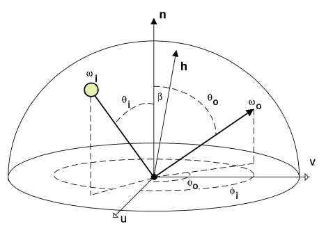
where all vectors are normalised. u is a vector in the surface plane. v is a vector in the surface plane orthogonal to u. n is the normal of the surface at p. β is the angle between n and h. The half vector h bisects the angle between the light source along ωi and view along ωo. Angle between ωi and n is θi. Angle between ωo and n is θo.
For some point p irradiated from all directions, the reflectance function determines the radiance coming from that point relative to some viewing direction. The function is
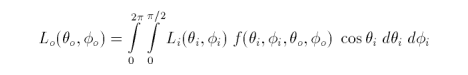
where L is the radiosity (i.e., irradiance) measured in watts per square metre (W/m2) and f is the BRDF. Azimuth (phi) is measured from the surface tangent vector u and elevation (theta) is measured from the surface normal n. The incoming and outgoing directions are denoted by the subscripts i and o, repsectively. For a single point light source, the equation becomes
![]()
The notation can be simplified if we represent the azimuth and elevation angles (both in radians) by the single term ω. Since all vectors in the BRDF model are normalised, the cosine term can be represented as a dot product.
![]()
This equation for total outgoing radiance is evaluated separately for each of the colour channels (as indicated with the component-wise multiplication of colour components in section 5.0.1.x).
Bidirectional reflectance distribution functions that are physically plausible obey the law of energy conservation. The law states that the quantity of energy reflected and/or scattered from a surface cannot exceed the original quantity of energy arriving at the surface. Mathematically, then,
![]()
must be equal to or less than one. These BRDFs also have the property of reciprocity. If the directions of the incoming and outgoing radiances were reversed, evaluating the BRDF will yield the same numerical value.
Shiny, curved objects have highlights when illuminated. A simplified BRDF that is fast to evaluate but not physically accurate for all shiny surface types is [38, 49]

where k is the specular reflection coefficient that varies in the range from zero to one. m is the specular colour component and mshine is the degree of shininess.
Most surfaces are not perfectly smooth. Microfacets were introduced into BRDF theory to model the imperfections of a given surface [40, 46, 51]. Each microfacet is a tiny, flat mirror on the surface, with a random size and orientation. Specular reflection is the result of direct reflections from a set of microfacets. Diffuse reflection is the result of the interreflection of light among several mircofacets. Because of the random nature of the mircofacets, some may either mask or even shadow other mircofacets. The BRDF, assuming specular reflection, is

F is the Fresnel term (see section 5.0.2 Fresnel Term for details). D is the Beckmann microfacet distribution function which defines the percentage of facets oriented in the direction of the half vector h. G is the geometric attenuation factor which defines the masking and shadowing of microfacets.

where m is the root-mean-square slope of the microfacets [7]. Large values of m indicate a steep slope and therefore more light is spread out; small values indicate a shallow slope where most of the microfacet normals are closely aligned with n, the normal of the surface. m can also be regarded as the roughness of the surface. β is the angle between n and h. The equation for G is

Here we take the minimum of the three values.
Diffuse surfaces reflect light equally in all directions in accordance to Lambert's Law of Reflection. As such, the BRDF always returns a constant value: the diffuse colour component m scaled by the diffuse reflection coefficient k.

Dusty surfaces scatter the reflected light in all directions toward grazing angles to the surface [45]. In this scenario, the BRDF is

An isotropic property of a surface is a property that behaves identically for all rotations around the surface normal. Properties that do, in fact, vary with respect to rotation around the surface normal are anisotropic. As such, visible light that strikes a surface may be reflected differently depending on the angle of incidence. To model this variance, robust BRDFs have been developed. For isotropic reflectance we have [52, 53]
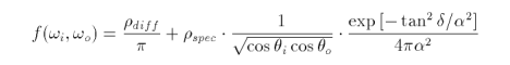
The rho values are the diffuse and specular reflectances. The delta value is the angle between the surface normal n and the half vector h. The alpha value is the standard deviation of the surface slope and should not be much greater than 0.2 [52].
An anisotropic reflectance model would use the following BRDF
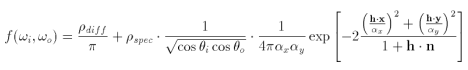
where the rho values are the diffuse and specular reflectances, x is a unit vector in the surface plane and y is the unit vector in the surface plane perpendicular to x. The standard deviations of the slope in the x and y directions are αx and αy respectively.
A dielectric material is one that becomes more reflective when viewed at progressively shallower angles. This phenomenon is called Fresnel reflectance and occurs when viewing materials such as plastics, glass or water. In computer graphics, the full Fresnel formula is simplified down to


where n is the index of refraction of the illuminated surface.
As paraphrased from the GNU General Public License "the following instances of program code are distributed in the hope that it will be useful, but without any warranty; without even the implied warranty of merchantability or fitness for a particular purpose." Please do not hesitate to notify me of any errors in logic and/or semantics.
// ----------------------------------------------------------
// brdf.h (basic framework only, no implementation)
// ----------------------------------------------------------

// The header file 'surface2.h' is available in section
// 3.1 Source Code
//

#ifndef __BRDF_H__
#define __BRDF_H__

#include <iostream>

#include "surface2.h"

class BRDF
{

   public:

      BRDF();
      ~BRDF();
      void *illuminate(Surface2 *, char);
      void setLight(double v[3], double c[4]);
      void setView(double v[3]);

      enum { BlinnPhong, CookTorrance, Lambertian,
             LommelSeeliger, WardIsotropic, WardAnisotropic };

  private:

      double lightVector[3];
      double viewVector[3];
      double colour[4];

};

inline void BRDF::setLight(double v[3], double c[4])
{

   lightVector[0] = v[0];
   lightVector[1] = v[1];
   lightVector[2] = v[2];

   colour[0] = c[0];
   colour[1] = c[1];
   colour[2] = c[2];
   colour[3] = c[3];

}

inline void BRDF::setView(double v[3])
{

   viewVector[0] = v[0];
   viewVector[1] = v[1];
   viewVector[2] = v[2];

}

#endif // __BRDF_H__


// ----------------------------------------------------------
// brdf.cpp (basic framework only, no implementation)
// ----------------------------------------------------------

// There are several APIs competing for mindshare in the
// realm of fragment shader programming.  Proprietary and/or
// open standards such as Cg, OpenGL 2.x and Direct3D (as
// part of DirectX 8.1 and later versions) all have pixel
// shader and vertex shader programming models.  Cg is a
// layer that can operate ontop of OpenGL and Direct3D.
//
// The following framework is just a very basic wrapper for
// the actual shader operations.
//

#include "brdf.h"

BRDF::BRDF() { }
BRDF::~BRDF() { }

void *BRDF::illuminate(Surface2 *s, char brdf)
{

   switch(brdf) {

   case BRDF::BlinnPhong: {
      break;
   }

   case BRDF::CookTorrance: {
      break;
   }

   case BRDF::Lambertian: {
      break;
   }

   case BRDF::LommelSeeliger: {
      break;
   }

   case BRDF::WardIsotropic: {
      break;
   }

   case BRDF::WardAnisotropic: {
      break;
   }

   default: {
      // use Lambertian BRDF
      //
      break;
   }

  }

  // some shader programming environments require you to
  // return a value.  the NULL result herein is just a
  // placeholder for the moment
  //

  return NULL;

}
[7] Foley, James D., Andries van Dam, Steven K. Feiner, and John F. Hughes,
Computer graphics: principles and practice (2nd ed.), Addison-Wesley
Longman Publishing Co., Inc., Boston, MA, 1990
[38] Blinn, James F., Models of Light Reflection for Computer Synthesised
Pictures, ACM Computer Graphics, SIGGRAPH 1977 Proceedings, 11(4):192-198
[39] Christensen, Per. H., Dani Lischinski, Eric J. Stollnitz and David
H. Salesin, Clustering for Glossy Global Illumination, ACM Transactions on
Graphics, 16(1):3-33, January 1997
[40] Cook, Robert L., and Kenneth E. Torrance, A Reflectance Model for Computer
Graphics, ACM Computer Graphics, SIGGRAPH 1981 Proceedings, 15(4):307-316
[41] Drettakis, George, and François X. Sillion, Interactive Update of Global
Illumination Using A Line-Space Hierarchy, ACM Computer Graphics, SIGGRAPH 1997
Proceedings, 31(4):57-64
[42] Dror, Ron O., Edward H. Adelson, and Alan S. Willsky, Estimating Surface
Reflectance Properties from Images under Unknown Illumination, Proceedings
of the SPIE 4299, Human Vision and Electronic Imaging IV, January 2001
[43] Fernandez, Sebastian, Kavita Bala, Moreno A. Piccolotto and Donald
P. Greenberg, Interactive Direct Lighting in Dynamic Scenes, Program of
Computer Graphics Technical Report: PCG-00-02, Cornell University, 2002
[44] Greger, Gene, Peter Shirley, Philip M. Hubbard and Donald P. Greenberg,
The Irradiance Volume, IEEE Computer Graphics and Applications, IEEE Inc.,
18(2):32-43, March 1998
[45] Hashemi, Leila, Ali Aziz and Mohammad Hasan Hashemi, Implementation of a
Single Photo Shape from Shading Method for the Automatic DTM Generation, PCV02
Photogrammetric Computer Vision, ISPRS Commission III, Symposium 2002
[46] Heidrich, Wolfgang and Hans-Peter Seidel, Realistic Hardware-accelerated
Shading and Lighting, ACM Computer Graphics, SIGGRAPH 1999 Proceedings,
33(4):57-64
[47] Kajiya, James T., The Rendering Equation, ACM Computer Graphics,
SIGGRAPH 1986 Proceedings, 20(4):143-150
[48] McAllister, David K., Anselmo Lastra and Wolfgang Heidrich, Efficient
Rendering of Spatial Bidirectional Reflectance Distribution Functions,
Graphics Hardware 2002, Eurographics/SIGGRAPH Workshop Proceedings,
September 2002
[49] Phong, Bui Tuong, Illumination of Computer-Generated Images, Department of
Computer Science, University of Utah, UTEC-CSs-73-129, July 1973
[50] Tole, Parag, Fabio Pellacini, Bruce Walter and Donald P. Greenberg,
Interactive Global Illumination in Dynamic Scenes, ACM Transactions on
Graphics 21(3):537-546, July 2002
[51] Torrance, Kenneth E., and E.M. Sparrow, Theory for off-specular reflection
from roughened surfaces, Journal of the Optical Society of America,
57(9):1105-1114, September 1967
[52] Ward, Gregory J., Measuring and Modeling Anistropic Reflection, ACM Computer
Graphics, SIGGRAPH 1992 Proceedings, 26(4):265-272
[53] Ward, Gregory J., The RADIANCE lighting simulation and rendering system,
ACM Computer Graphics, SIGGRAPH 1994 Proceedings, 28(4):459-472
2003.02.04
Wavelets are used to represent functions in an elegant manner. The function can be an image, curve or surface. With its initial use in approximation theory and signal processing [61, 59], wavelets can also be applied to image editing [64], global illumination [54, 60], radiosity [57] and surface reconstruction [55, 56, 58]. In this introduction to wavelets, it's assumed the reader is familiar with concepts associated with linear algebra.
Suppose we have a sequence of four grid cells where each cell is assigned a value in the range from zero to 15. We can represent this sequence in several ways. For this discussion, we will simply use a single row of numbers.
![]()
Averaging these values, pairwise, yields the sequence
![]()
Any lost information, due to decomposition, is captured in detail coefficients. The first coefficient is three (3) because the first pairwise average is three less than 15 and three more than nine. The second coefficient is negative one, since 2 + (-1) = 1 and 2 - (-1) = 3. Applying the procedure recursively gives a full decomposition of the function.
| Resolution | Averages | Detail Coefficients |
|---|---|---|
| 4 | [ 15 9 1 3 ] | |
| 2 | [ 12 2 ] | [ 3 -1 ] |
| 1 | [ 7 ] | [ 5 ] |
The wavelet transform of our original four-value sequence is the single coeffecient representing the overall average of values followed by the detail coefficients in order of increasing resolution.
![]()
The process to create the wavelet transform is called a filter bank [63]. The transform is used to reconstruct the original sequence to any resolution by recursively adding or subtracting the detail coefficients, along with constant offsets to these coefficients, from a lower resolution. An implementation of the filter bank (for both decomposing and reconstruction) is available in section 6.1 Source Code.
Instead of a sequence of numbers, suppose we represent our original sequence as a series of constant functions that all fit within the open interval [0, 1). In our example, we have four grid cells so the support of each constant function must therefore be 1/4.
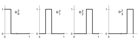
These four (4 = 22) box functions are known as the Haar basis of the vector space V2. Each member of the Haar basis is known as a scaling function and is defined thusly,
![]()
where

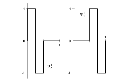
Functions in Vn+1 that are orthogonal to functions in Vn define vector space Wn. Haar wavelets are those functions that span W. These wavelets are defined thusly,
![]()
where

The Haar wavelets that span W1 and correspond to the basis in V1 are
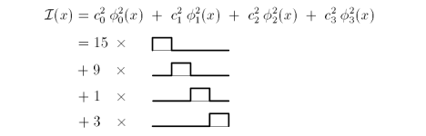
With scaling functions φ and Haar wavelets ψ, we can express a discrete function as a linear combination of these bases [63].
Our original sequence of values as a linear combination of scaling functions in V2, is
In terms of functions in V1 and W1 we have
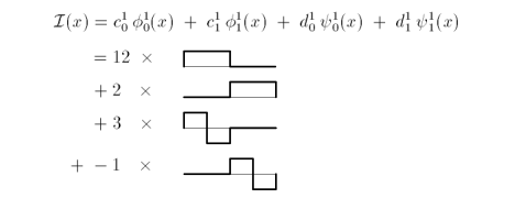
Using V0, W0 and W1 the wavelet transform is
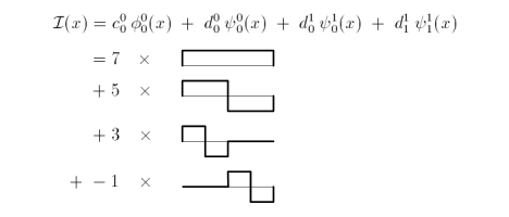
From these expressions of our discrete function, at varying resolutions, we see that 'c' are the pairwise averages and 'd' are the detail coefficients.
| Vector spaces | Resolution | Haar basis coefficients | Haar wavelet coefficients |
| V2, W2 | 22 | [ 15 9 1 3 ] | |
| V1, W1 | 21 | [ 12 2 ] | [ 3 -1 ] |
| V0, W0 | 20 | [ 7 ] | [ 5 ] |
As paraphrased from the GNU General Public License "the following instances of program code are distributed in the hope that it will be useful, but without any warranty; without even the implied warranty of merchantability or fitness for a particular purpose." Please do not hesitate to notify me of any errors in logic and/or semantics.
// ----------------------------------------------------------
// filterBank.h
// ----------------------------------------------------------

#ifndef __FILTER_BANK_H__
#define __FILTER_BANK_H__

#include <iostream>

#include <map>

class FilterBank
{

   public:

      FilterBank();
      ~FilterBank();
      map<int, double> decompose(map<int, double>);
      map<int, double> reconstruct(map<int, double>);

   private:

      map<int, double> decomposeStep(map<int, double>, int);
      map<int, double> reconstructStep(map<int, double>, int);

};

#endif // __FILTER_BANK_H__

// ----------------------------------------------------------
// filterBank.cpp
// ----------------------------------------------------------

#include "filterBank.h"

FilterBank::FilterBank() { }
FilterBank::~FilterBank() { }

map<int, double> FilterBank::decompose(map<int, double> c)
{

   int g;

   g = c.size();
   while (g >= 2) {
      c = decomposeStep(c, g);
      g /= 2;
   }

   return c;

}

map<int, double>

FilterBank::decomposeStep(map<int, double> c, int g)
{

   int i;
   int j;
   map<int, double> cc = c;

   j = g / 2;

   // perform pairwise averaging to decompose original data
   //

   for (i=1; i<=j; ++i) {
      cc[i] = (c[2*i - 1] + c[2*i]) * 0.5;
      cc[j + i] = (c[2*i - 1] - c[2*i]) * 0.5;
   }

   return cc;

}

map<int, double> FilterBank::reconstruct(map<int, double> c)
{

    int g;
    int h;

    h = c.size();

    g = 2;
    while (g <= h) {
       c = reconstructStep(c, g);
       g *= 2;
    }

    return c;

}

map<int, double>

FilterBank::reconstructStep(map<int, double> c, int g)
{

   int i;
   int j;
   map<int, double> cc = c;

   j = g / 2;

   // add detail coefficients to reconstruct original data
   //

   for (i=1; i<=j; ++i) {
      cc[2*i - 1] = c[i] + c[j + i];
      cc[2*i] = c[i] - c[j + i];
   }

   return cc;

}


// ----------------------------------------------------------
// filterBank2D.h
// ----------------------------------------------------------

#ifndef __FILTER_BANK2D_H__
#define __FILTER_BANK2D_H__

#include <iostream>
#include <map>

class FilterBank2D
{

   public:

      FilterBank2D();
      ~FilterBank2D();
      map<int, double> decompose(map<int, double>);
      map<int, double> reconstruct(map<int, double>);
      void setLength(int);
      int getLength(void);

   private:

      map<int, double> decomposeRow(map<int, double>, int, int);
      map<int, double> decomposeCol(map<int, double>, int, int);

      map<int, double> reconstructCol(map<int, double>, int, int);
      map<int, double> reconstructRow(map<int, double>, int, int);

      int length;

};

inline void FilterBank2D::setLength(int a)
{

   if ((a % 2) != 0) --a;
   length = (a > 1) ? a : 2;

}

inline int FilterBank2D::getLength(void)
{

   return length;

}

#endif // __FILTER_BANK2D_H__

// ----------------------------------------------------------
// filterBank2D.cpp
// ----------------------------------------------------------

#include "filterBank2D.h"

FilterBank2D::FilterBank2D()
{

   length = 2;

}

FilterBank2D::~FilterBank2D() { }

map<int, double> FilterBank2D::decompose(map<int, double> c)
{

   // c = square matrix in row-major order; c[0] is not used

   int i;
   int g;
   int row, col;

   g = length;
   while (g >= 2) {

      for (row=1; row<=g; ++row) {

         c = decomposeRow(c, g, row);

      }

      for (col=1; col<=g; ++col) {

         c = decomposeCol(c, g, col);

      }

      g /= 2;

   }

   return c;

}

map<int, double>

FilterBank2D::decomposeRow(map<int, double> c, int g, int row)
{

   int i, j;
   int offset;
   map<int, double> cc, cd;

   i = 1;
   offset = (row - 1) * length + 1;
   while (i<=length) {

      cd[i] = cc[i] = c[offset];
      ++offset;
      ++i;

   }

   i = 1;
   j = g / 2;
   while (i<=j) {

      cc[i] = (cd[2*i - 1] + cd[2*i]) * 0.5;
      cc[j + i] = (cd[2*i - 1] - cd[2*i]) * 0.5;
      ++i;

   }

   i = 1;
   offset = (row - 1) * length + 1;
   while (i<=length) {

      c[offset] = cc[i];
      ++offset;
      ++i;

   }

   return c;

}

map<int, double>
FilterBank2D::decomposeCol(map<int, double> c, int g, int col)
{

   int i, j;
   int offset;
   map<int, double> cc, cd;

   i = 1;
   offset = col;
   while (i<=length) {

      cd[i] = cc[i] = c[offset];
      offset += length;
      ++i;

   }

   i = 1;
   j = g / 2;
   while (i<=j) {

      cc[i] = (cd[2*i - 1] + cd[2*i]) * 0.5;
      cc[j + i] = (cd[2*i - 1] - cd[2*i]) * 0.5;
      ++i;

   }

   i = 1;
   offset = col;
   while (i<=length) {

      c[offset] = cc[i];
      offset += length;
      ++i;

   }

   return c;

}

map<int, double> FilterBank2D::reconstruct(map<int, double> c)
{

   // c = square matrix in row-major order; c[0] is not used

   int i;
   int g, h;
   int row, col;

   h = length;

   g = 2;
   while (g <= h) {

      for (col=1; col<=g; ++col) {

         c = reconstructCol(c, g, col);

      }

      for (row=1; row<=g; ++row) {

         c = reconstructRow(c, g, row);

      }

      g *= 2;

   }

   return c;

}

map<int, double>

FilterBank2D::reconstructCol(map<int, double> c, int g, int col)
{

   int i, j;
   int offset;
   map<int, double> cc, cd;

   i = 1;
   offset = col;
   while (i<=length) {

      cd[i] = cc[i] = c[offset];
      offset += length;
      ++i;

   }

   i = 1;
   j = g / 2;
   while (i<=j) {

      cc[2*i - 1] = cd[i] + cd[j + i];
      cc[2*i] = cd[i] - cd[j + i];
      ++i;

   }

   i = 1;
   offset = col;
   while (i<=length) {

      c[offset] = cc[i];
      offset += length;
      ++i;

   }

   return c;

}

map<int, double>
FilterBank2D::reconstructRow(map<int, double> c, int g, int row)
{

   int i, j;
   int offset;
   map<int, double> cc, cd;

   i = 1;
   offset = (row - 1) * length + 1;
   while (i<=length) {

      cd[i] = cc[i] = c[offset];
      ++offset;
      ++i;

   }

   i = 1;
   j = g / 2;
   while (i<=j) {

      cc[2*i - 1] = cd[i] + cd[j + i];
      cc[2*i] = cd[i] - cd[j + i];
      ++i;

   }

   i = 1;
   offset = (row - 1) * length + 1;
   while (i<=length) {

      c[offset] = cc[i];
      ++offset;
      ++i;

   }

   return c;

}
[54] Christensen, Per H., Eric J. Stollnitz, David H. Salesin and Tony
D. DeRose, Global Illumination of Glossy Environments Using Wavelets and
Importance, ACM Transactions On Graphics, Association of Computing
Machinery, 15(1):37-71, January 1996
[55] Gortler, S.J., Wavelet Methods for Computer Graphics, TR-477-94, Ph.D.
dissertation, Department of Computer Science, Princeton University,
January 1995
[56] Gortler, S.J., and Michael F. Cohen, Variational Modeling With Wavelets,
TR-456-94, Department of Computer Science, Princeton University,
April 1994
[57] Gortler, S.J., Peter Schröder, Michael F. Cohen, and Pat
Hanrahan, Wavelet Radiosity, ACM Computer Graphics, SIGGRAPH 1993
Proceedings, 27(4):221-230
[58] Gross, M.H., O.G. Staadt, and R. Gatti, Efficient Triangular Surface
Approximations Using Wavelets and Quadtree Data Structures, IEEE
Transactions on Visualisation and Computer Graphics, 2(2):130-143,
June 1996
[59] Jameson, Leland, Wavelet-based Grid Generation, Institute for Computer
Applications in Science and Engineering, NASA Langley Research Centre,
CR-201609 ICASE Report, No. 96-59, October 1996
[60] Lewis, Robert R., Wavelet Radiative Transfer and Surface Interaction,
TR-96-07, Imager Computer Graphics Lab, University of British Columbia,
Department of Computer Science, February 1996
[61] Mallat, S., A Theory for Multiresolution Signal Decomposition:
The Wavelet Representation, IEEE Transactions on Pattern Analysis and
Machine Intelligence, 11(7):674-693, July 1989
[62] Schröder, Peter and Wim Sweldens, Spherical Wavelets: Efficiently
Representing Functions on the Sphere, ACM Computer Graphics, SIGGRAPH 1995
Proceedings, 29(4):161-172
[63] Stollnitz, Eric J., Tony D. DeRose and David H. Salesin, Wavelets for
Computer Graphics: A Primer, Part 1, IEEE Computer Graphics and Applications,
IEEE Inc., 15(3):76-84
[64] Stollnitz, Eric J., Tony D. DeRose and David H. Salesin, Wavelets for
Computer Graphics: A Primer, Part 2, IEEE Computer Graphics and Applications,
IEEE Inc., 15(4):75-85