More than one patch is often required to adaquately describe the complexities of an object. This piece-wise approach has several benefits, one of which is the ability to stitch together simple patches that are easy to manipulate and fast to draw. The artist also has the freedom to edit parts of the composite surface without having to worry about global side-effects. For this discussion, it's assumed the reader is familiar with Bézier forms [21] and the concepts introduced in Tessellation.

The system of patches may consist of surfaces with different degrees and varying tessellation requirements. A patch that is planar will only need sparse sampling. In areas of curvature we want more samples to better represent smoothness. A comprehensive evalution method is therefore needed to ensure patches of all types are properly tessellated. The method chosen herein is called central differencing. The derivation of the formulae is straightfoward but tedious. Those wishing to delve into the details should have a look at the appendix section entitled Central Differencing.

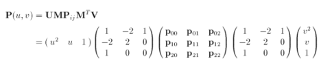
The parametric equation of a biquadratic Bézier surface written in matrix form is

The setup information we need to evaluate the surface is

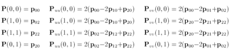
and

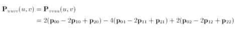
where u = 0, 1 and v = 0, 1. After this initialisation we are ready to calculate the surface points via central differencing. As we split the surface, we bisect a curve along constant u. The result of this split is a midpoint M and its corresponding second partial derivates. In the next phase of the subdivision, M is used as the endpoint for a curve to be split along constant v. The process continues recursively until some predefined limit. Looking at this another way, we split a patch in half along one axis to create a 'left' subpatch and a 'right' subpatch. We then take each of these subpatches and split them in half along the other axis. Creating and splitting subsequent subpatches is the basic premise of this method. The psuedocode to evaluate the surface is.

let uL = upper left corner of the patch
let lL = lower left corner of the patch
let uR = upper right corner of the patch
let lR = lower right corner of the patch

let patch  = uL, uR, lL, lR
let uSplit = true

let k = 0.5
let E = a very small number less than k

for each of the four corners of the patch, compute P and
the second partial derivatives in both u and v

function centralDiff(patch, k, uSplit)

if (k is less than E) return

if (uSplit) {

along constant v
let uM = midPoint of [uL, uR]
let lM = midPoint of [lL, lR]
let uSplit = false

} else {

along constant u
let uM = midPoint of [uL, uR]
let lM = midPoint of [lL, lR]
let uSplit = true

}

if [uL, uM, uR] are not collinear
display uM

if [lL, lM, lR] are not collinear
display lM

at alternate subdivision level let k = k * 0.5
centralDiff(left  subpatch, k, uSplit)
centralDiff(right subpatch, k, uSplit)

done

Section 3.1 Source Code has a full implementation of the evaluation method.

Suppose we want to join two surfaces along a common border. Gaps will appear at the interface if one surface is tessellated at a higher frequency than the other surface. One simple way to reduce the occurance of visible seams between surfaces is to ensure both patches share the same points along the common edge. The algorithm, known as fractional tessellation, involves modifying the sampling density along the shared edge [28].

Many physics and illumination models require normals at each surface point. The calculations are highly sensitive to any discontinuities. Such differences are most glaring along the interface of two patches. To ensure a smooth transition from one patch to another, the pair of rows (or columns) of control points that are closest to the shared edge must be adjusted to minimise abrupt changes.

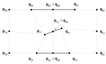
Enforcing this parametric continuity requires us to make certain that the direction and magnitude of the first derivatives at the control points along the border are equal [21]. In others words, given two biquadratic surfaces P and Q joined along one edge, the following equation must be satisfied

where j varies in the range from zero to one. Such a condition is achieved if each of the following triplets of control points are collinear (see bold line segments in diagram).

and

where k is a constant [1]. An algorithm that stitches together two patches must edit the control nets, if necessary, before surface evaluation. Stitching together four patches to share a corner point requires parametric continuity in both u and v.

As paraphrased from the GNU General Public License "the following instances of program code are distributed in the hope that it will be useful, but without any warranty; without even the implied warranty of merchantability or fitness for a particular purpose." Please do not hesitate to notify me of any errors in logic and/or semantics.

// ----------------------------------------------------------
// surface2.h (for biquadratic surfaces only)
// ----------------------------------------------------------

#ifndef __SURFACE2_H__
#define __SURFACE2_H__

#include <iostream>

using namespace std;

typedef struct {

double x, y, z;

} Point;

typedef struct {

double p[3];
double uu[3];
double vv[3];
double uuvv[3];
double vvuu[3];

} Point2;

class Surface2
{

public:

Surface2(Point [3][3]);
~Surface2();
void draw(int);

private:

void init(Point2 *, Point2 *, Point2 *, Point2 *);
void subdivide(Point2 *, Point2 *, Point2 *, Point2 *,
	     double, char, char);

char collinear(double [3], double [3], double[3]);
void plot(Point2);

double min;
Point P[3][3];

};


#endif // __SURFACE2_H__

// ----------------------------------------------------------
// surface2.cpp (for biquadratic surfaces only)
// ----------------------------------------------------------

#include "surface2.h"

Surface2::Surface2(Point c[][3])
{

int i, j;

for (i=0;i<3;++i) {
for (j=0;j<3; ++j) {
 P[i][j].x = c[i][j].x;
 P[i][j].y = c[i][j].y;
 P[i][j].z = c[i][j].z;
}
}

}


Surface2::~Surface2() { }

void Surface2::draw(int steps)
{

Point2 uL, uR, lL, lR;

init(&uL, &uR, &lL, &lR);

if (steps < 2) return;
if ((steps % 2) != 0) ++steps;

min = 1.0 / (double)(steps << 1);
subdivide(&uL, &uR, &lL, &lR, 0.5, 1, 0);

}

void Surface2::subdivide(Point2 *uL, Point2 *uR, Point2 *lL,
		 Point2 *lR, double k, char uSplit,
		 char c)
{

// the following evaluator code may look rather complex
// but it's more efficient than direct evaluation of the
// biquadratic surface equation.
//
// a maximum of two samples are plotted for each call
// to subdivide().
//
// the midPoint lM along the shared edge of two subpatches
// may be generated twice
//


Point2 uM;   // midpoint along [uL, uR]
Point2 lM;   // midpoint along [lL, lR]
double k2;

if (k < min) return;
k2 = k*k;

if (uSplit) {

uM.uu[0] = (uL->uu[0] + uR->uu[0]) * 0.5;
uM.uu[1] = (uL->uu[1] + uR->uu[1]) * 0.5;
uM.uu[2] = (uL->uu[2] + uR->uu[2]) * 0.5;

uM.uuvv[0] = uM.vvuu[0] = (uL->uuvv[0] + uR->uuvv[0]) * 0.5;
uM.uuvv[1] = uM.vvuu[1] = (uL->uuvv[1] + uR->uuvv[1]) * 0.5;
uM.uuvv[2] = uM.vvuu[2] = (uL->uuvv[2] + uR->uuvv[2]) * 0.5;

uM.p[0] = (uL->p[0] + uR->p[0] - k2*uM.uu[0]) * 0.5;
uM.p[1] = (uL->p[1] + uR->p[1] - k2*uM.uu[1]) * 0.5;
uM.p[2] = (uL->p[2] + uR->p[2] - k2*uM.uu[2]) * 0.5;

uM.vv[0] = (uL->vv[0] + uR->vv[0] - k2*uM.uuvv[0]) * 0.5;
uM.vv[1] = (uL->vv[1] + uR->vv[1] - k2*uM.uuvv[1]) * 0.5;
uM.vv[2] = (uL->vv[2] + uR->vv[2] - k2*uM.uuvv[2]) * 0.5;

lM.uu[0] = (lL->uu[0] + lR->uu[0]) * 0.5;
lM.uu[1] = (lL->uu[1] + lR->uu[1]) * 0.5;
lM.uu[2] = (lL->uu[2] + lR->uu[2]) * 0.5;

lM.uuvv[0] = lM.vvuu[0] = (lL->uuvv[0] + lR->uuvv[0]) * 0.5;
lM.uuvv[1] = lM.vvuu[1] = (lL->uuvv[1] + lR->uuvv[1]) * 0.5;
lM.uuvv[2] = lM.vvuu[2] = (lL->uuvv[2] + lR->uuvv[2]) * 0.5;

lM.p[0] = (lL->p[0] + lR->p[0] - k2*lM.uu[0]) * 0.5;
lM.p[1] = (lL->p[1] + lR->p[1] - k2*lM.uu[1]) * 0.5;
lM.p[2] = (lL->p[2] + lR->p[2] - k2*lM.uu[2]) * 0.5;

lM.vv[0] = (lL->vv[0] + lR->vv[0] - k2*lM.uuvv[0]) * 0.5;
lM.vv[1] = (lL->vv[1] + lR->vv[1] - k2*lM.uuvv[1]) * 0.5;
lM.vv[2] = (lL->vv[2] + lR->vv[2] - k2*lM.uuvv[2]) * 0.5;

uSplit = 0;

} else {

uM.vv[0] = (uL->vv[0] + uR->vv[0]) * 0.5;
uM.vv[1] = (uL->vv[1] + uR->vv[1]) * 0.5;
uM.vv[2] = (uL->vv[2] + uR->vv[2]) * 0.5;

uM.vvuu[0] = uM.uuvv[0] = (uL->vvuu[0] + uR->vvuu[0]) * 0.5;
uM.vvuu[1] = uM.uuvv[1] = (uL->vvuu[1] + uR->vvuu[1]) * 0.5;
uM.vvuu[2] = uM.uuvv[2] = (uL->vvuu[2] + uR->vvuu[2]) * 0.5;

uM.p[0] = (uL->p[0] + uR->p[0] - k2*uM.vv[0]) * 0.5;
uM.p[1] = (uL->p[1] + uR->p[1] - k2*uM.vv[1]) * 0.5;
uM.p[2] = (uL->p[2] + uR->p[2] - k2*uM.vv[2]) * 0.5;

uM.uu[0] = (uL->uu[0] + uR->uu[0] - k2*uM.vvuu[0]) * 0.5;
uM.uu[1] = (uL->uu[1] + uR->uu[1] - k2*uM.vvuu[1]) * 0.5;
uM.uu[2] = (uL->uu[2] + uR->uu[2] - k2*uM.vvuu[2]) * 0.5;

lM.vv[0] = (lL->vv[0] + lR->vv[0]) * 0.5;
lM.vv[1] = (lL->vv[1] + lR->vv[1]) * 0.5;
lM.vv[2] = (lL->vv[2] + lR->vv[2]) * 0.5;

lM.vvuu[0] = lM.uuvv[0] = (lL->vvuu[0] + lR->vvuu[0]) * 0.5;
lM.vvuu[1] = lM.uuvv[1] = (lL->vvuu[1] + lR->vvuu[1]) * 0.5;
lM.vvuu[2] = lM.uuvv[2] = (lL->vvuu[2] + lR->vvuu[2]) * 0.5;

lM.p[0] = (lL->p[0] + lR->p[0] - k2*lM.vv[0]) * 0.5;
lM.p[1] = (lL->p[1] + lR->p[1] - k2*lM.vv[1]) * 0.5;
lM.p[2] = (lL->p[2] + lR->p[2] - k2*lM.vv[2]) * 0.5;

lM.uu[0] = (lL->uu[0] + lR->uu[0] - k2*lM.vvuu[0]) * 0.5;
lM.uu[1] = (lL->uu[1] + lR->uu[1] - k2*lM.vvuu[1]) * 0.5;
lM.uu[2] = (lL->uu[2] + lR->uu[2] - k2*lM.vvuu[2]) * 0.5;

uSplit = 1;

}

if ( !collinear(uL->p, uM.p, uR->p) ) plot(uM);
if ( !collinear(lL->p, lM.p, lR->p) ) plot(lM);

++c;
if ((c % 2) == 0) k = k * 0.5;
subdivide(lL, uL, &lM, &uM, k, uSplit, c);
subdivide(uR, lR, &uM, &lM, k, uSplit, c);

}

void Surface2::init(Point2 *uL, Point2 *uR,
	    Point2 *lL, Point2 *lR)
{

uL->p[0] = P[0][0].x;
uL->p[1] = P[0][0].y;
uL->p[2] = P[0][0].z;

uL->uu[0] = 2*(P[0][0].x - 2*P[1][0].x + P[2][0].x);
uL->uu[1] = 2*(P[0][0].y - 2*P[1][0].y + P[2][0].y);
uL->uu[2] = 2*(P[0][0].z - 2*P[1][0].z + P[2][0].z);

uL->vv[0] = 2*(P[0][0].x - 2*P[0][1].x + P[0][2].x);
uL->vv[1] = 2*(P[0][0].y - 2*P[0][1].y + P[0][2].y);
uL->vv[2] = 2*(P[0][0].z - 2*P[0][1].z + P[0][2].z);

uL->uuvv[0] = uL->vvuu[0] =
uL->uu[0] - 4*(P[0][1].x - 2*P[1][1].x + P[2][1].x) +
2*(P[0][2].x - 2*P[1][2].x + P[2][2].x);

uL->uuvv[1] = uL->vvuu[1] =
uL->uu[1] - 4*(P[0][1].y - 2*P[1][1].y + P[2][1].y) +
2*(P[0][2].y - 2*P[1][2].y + P[2][2].y);

uL->uuvv[2] = uL->vvuu[2] =
uL->uu[2] - 4*(P[0][1].z - 2*P[1][1].z + P[2][1].z) +
2*(P[0][2].z - 2*P[1][2].z + P[2][2].z);

plot(*uL);

//

uR->p[0] = P[0][2].x;
uR->p[1] = P[0][2].y;
uR->p[2] = P[0][2].z;

uR->uu[0] = uL->uu[0];
uR->uu[1] = uL->uu[1];
uR->uu[2] = uL->uu[2];

uR->vv[0] = 2*(P[2][0].x - 2*P[2][1].x + P[2][2].x);
uR->vv[1] = 2*(P[2][0].y - 2*P[2][1].y + P[2][2].y);
uR->vv[2] = 2*(P[2][0].z - 2*P[2][1].z + P[2][2].z);

uR->uuvv[0] = uR->vvuu[0] = uL->uuvv[0];
uR->uuvv[1] = uR->vvuu[1] = uL->uuvv[1];
uR->uuvv[2] = uR->vvuu[2] = uL->uuvv[2];

plot(*uR);

//

lL->p[0] = P[2][0].x;
lL->p[1] = P[2][0].y;
lL->p[2] = P[2][0].z;

lL->uu[0] = 2*(P[0][2].x - 2*P[1][2].x + P[2][2].x);
lL->uu[1] = 2*(P[0][2].y - 2*P[1][2].y + P[2][2].y);
lL->uu[2] = 2*(P[0][2].z - 2*P[1][2].z + P[2][2].z);

lL->vv[0] = uL->vv[0];
lL->vv[1] = uL->vv[1];
lL->vv[2] = uL->vv[2];

lL->uuvv[0] = lL->vvuu[0] = uL->uuvv[0];
lL->uuvv[1] = lL->vvuu[1] = uL->uuvv[1];
lL->uuvv[2] = lL->vvuu[2] = uL->uuvv[2];

plot(*lL);

//

lR->p[0] = P[2][2].x;
lR->p[1] = P[2][2].y;
lR->p[2] = P[2][2].z;

lR->uu[0] = lL->uu[0];
lR->uu[1] = lL->uu[1];
lR->uu[2] = lL->uu[2];

lR->vv[0] = uR->vv[0];
lR->vv[1] = uR->vv[1];
lR->vv[2] = uR->vv[2];

lR->uuvv[0] = lR->vvuu[0] = uL->uuvv[0];
lR->uuvv[1] = lR->vvuu[1] = uL->uuvv[1];
lR->uuvv[2] = lR->vvuu[2] = uL->uuvv[2];

plot(*uR);

}

char Surface2::collinear(double a[3], double b[3], double c[3])
{

double d, r[3], s[3], t[3];

r[0] = a[0] - b[0];
r[1] = a[1] - b[1];
r[2] = a[2] - b[2];

s[0] = c[0] - b[0];
s[1] = c[1] - b[1];
s[2] = c[2] - b[2];

t[0] = r[1]*s[2] - s[1]*r[2];
t[1] = s[0]*r[2] - r[0]*s[2];
t[2] = r[0]*s[1] - s[0]*r[1];

d = t[0]*t[0] + t[1]*t[1] + t[2]*t[2];
return ((d > -0.001 && d < 0.001) ? 1 : 0);

}

void Surface2::plot(Point2 T)
{

// the spatial coordinates of the surface point is
// (T.p[0], T.p[1], T.p[2])
//

}

[1] Akenine-Möller, Tomas and Eric Haines, Real-Time Rendering 2nd. Ed., A.K. Peters Ltd, 2002
[21] Farin, G., Curves and Surfaces for Computer-Aided Geometric Design: A Practical Guide, Fourth Edition, Academic Press, San Diego, 1997
[28] Moreton, H., Watertight Tessellation using Forward Differencing, ACM SIGGRAPH/Eurographics Workshop on Graphics Hardware, pp 25-132, August 2001

Articles | Contact

A photon is a quantum of electromagnetic energy. We perceive this energy as visible light if its wavelength falls within the range of four thousand (violet) to eight thousand (red) angstroms. To simulate an outdoor environment we often use the Sun as the light source. The Sun, in our model, is a directional light source as is the Moon. The contributions of the stars, planets, zodiacal light, airglow, and diffuse galactic and cosmic light are also important if we wish to accurately portray an outdoor setting [31]. These sources are assumed to be infinitely far away from the scene being lit. This assumption allows us to simplify our lighting model.

The illumination i at each point on a surface is calculated using a lighting model. This model consists of three components: ambient, diffuse and specular. When added together, these components yield a final colour. Our lighting model is not based on the actual physical behaviour of light and its interactions with solids. Instead we will make several generalisations that produce a fairly good representation of reality.

Since the final colour itotal is the sum of three components

the situation may arise where the red, green or blue colour components are greater than one. In this case, we simply scale all values against the highest value. If, for example, the final colour is defined as a very bright red (4.5, 1.0, 0.8) we simply scale the colour components by 1/4.5 to arrive at (1.0, 0.222, 0.178). We perform this scaling in order to preserve the original hue and saturation.

The geometry of our lighting model is

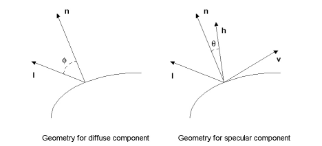
n is the surface normal, l is the light vector, v is the view vector and h bisects the angle between l and v. All vectors in our model are normalised.

The light that falls upon an object comes from all directions: directly from light sources and also indirectly when light bounces off surfaces before reaching the object. To represent this ambient light, our lighting model includes the ambient component iamb

m represents the intrinsic material colour of the object. The quantity has three components: red, green and blue. s represents the colour of the light source which is also defined by three colour components. The operator between these values is a component-wise multiplication. If, for example, a red object m = (1.0, 0.0, 0.0) is illuminated by a green light source s = (0.0, 1.0, 0.0), we will preceive the ambient light radiating from the object as black i = (0.0, 0.0, 0.0). In other words, the red object absorbs the green light. Component-wise multiplication yields colour components in the range from zero to one.

According to Lambert's Law, for portions of a surface that are ideally diffuse (i.e., not shiny), the reflected light is determined by the cosine between the surface normal n and the light vector l.

Since all vectors in our lighting model are normalised, the equation for the diffuse component idiff can be rewritten as

The quantities m and s represent the intrinsic diffuse colour of the material and the light source, respectively.

Shiny, curved objects have highlights when illuminated. To simulate these highlights our lighting model consists of the specular component ispec

The quantities m and s represent the intrinsic specular colour of the material and the light source, respectively. n is the surface normal and h is the half vector that bisects the angle between the light vector l and the view vector v. The shininess of the object is represented by mshine. More shiny objects have greater values of mshine.

The typical irradiance from the Sun is 620 000 times greater than all other celesital bodies, combined, when measured by an Earth-bound observer [32]. The Sun is the main source of ambient and diffuse lighting in our model during the day. At night, the contributors of natural light are the Moon, zodical light and starlight. Airglow, diffuse galactic light and cosmic light are evident only during the most ideal of nightime conditions. This assumes, of course, that the sky overhead is not obscured too greatly by clouds or other dense particle formations.

Sky colour, the result of sunlight intersecting the upper layers of the atmosphere, is the ambient colour that irradiates an outdoor environment during the daylight hours. The determination of sky colour should take into account multiple scattering effects of sunlight due to air molecules, dust particles, mixed gases, water vapour and other aerosols [33, 34, 35, 36, 37]. Robust methods to calculate sky colour and the colour of sunlight at different elevations handle light in terms of wavelength and colour spaces sanctioned by the Commission Internationale de l'Éclairage (CIE). The values are then converted to RGB colour space for display.

To calculate the postion of the Sun in spherical coordinates relative to an observer on Earth at p requires several equations [36]. First, we need to determine the solar time t (in decimal hours) from standard time ts (in decimal hours) using

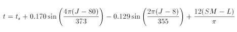
where SM is the standard meridian for the time zone in radians. L is the longitude, in radians, at p. Solar declination, measured in radians, is

J is the Julian date (i.e., the day of the year as an integer in the range from one to 365 inclusive). The solar position we want in terms of zenith and azimuth angles, for Earth-bound observers, is

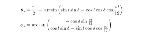
where l is the latitude in radians at p. The zenith angle (theta) ranges from from 0 to π/2. Angles greater than π/2 are below the horizon. Positive values for the azimuthal angle (phi) represent direction west of south.

For nighttime scenes of outdoor environments, natural illumination is an important factor for the creation of realistic images [31]. Models for moonlight, night skylight and starlight are used to yield the proper tone reproduction we observe with the naked eye [32]. At night, we preceive a 'blue-shift' of colours and a loss of detail. Jensen, et. al., simulated the shift in hue by working in CIE XYZV colour space. A blur that is variant to spatial coordinates is used to approximate the loss of detail and is applied on a per-texel basis. The calculations to yield the colour shifted XYZV values at each image grid cell are:

The value at each grid cell in CIE XYZV colour space is then converted to RGB colour space for display.

During the day, the sky is never uniform in colour. The luminance of the sky at any given view direction v depends on two factors: the luminance at the zenith (i.e., directly overhead) and the sky luminance distribution function [36]. Our sky model uses these variables to accurately render the proper colours of the hemisphere that surrounds the viewer at p. The hemisphere is partitioned into a series of quads known as sky elements. The geometry of our model is

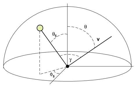
where θ is the angle from the zenith to v. The gamma term is the angle between v and direction toward the Sun located at (θs, φs).

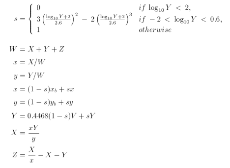
Our sky model operates within the CIE XYZ colour space. To simplify the calculations, we will ignore the multiple scattering effects of sunlight due to air molecules, dust particles, mixed gases, water vapour and other aerosols. The luminance variable CIE Y and chromaticities x and y for a sky element are determined thusly [36].

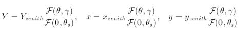
where

Preetham et. al., published values for luminance and chromaticities at the zenith, and typical values for the distribution coefficients A, B, C, D and E [36]. The coefficients are unique for Y, x and y. From these results we then compute the CIE X, Y and Z values for the sky element as seen along v where

We then perform the CIE XYZ to RGB conversion and the render the sky element accordingly. We scale the RGB triplet if any of its components is greater than one. Section 4.1 Source Code has an implementation of the sky model sans the actual rendering step. Each sky element is a diffuse light source which contributes to the overall colour of the surfaces at p.

As paraphrased from the GNU General Public License "the following instances of program code are distributed in the hope that it will be useful, but without any warranty; without even the implied warranty of merchantability or fitness for a particular purpose." Please do not hesitate to notify me of any errors in logic and/or semantics.

// ----------------------------------------------------------
// sun.h
// ----------------------------------------------------------

#ifndef __SUN_H__
#define __SUN_H__

#include <iostream>
#include <math.h>

class Sun
{

public:

Sun();
~Sun();

void calculatePosition(double, double, double, double,
		    int);

void setColour(double [4]);
double getTheta(void);
double getPhi(void);

private:

double theta;   // angle from surface normal
	      // 0 = directly overhead
	      // pi/2 = at horizon

double phi;     // angle from south direction
	      // 0 = south
	      // pi/2 = west
	      // -pi/2 = east

double colour[4];

};

inline void Sun::setColour(double c[4])
{

colour[0] = c[0];
colour[1] = c[1];
colour[2] = c[2];
colour[3] = c[3];

}

inline double Sun::getTheta()
{

return theta;

}

inline double Sun::getPhi()
{

return phi;

}

#endif // __SUN_H__

// ----------------------------------------------------------
// sun.cpp
// ----------------------------------------------------------

#include "sun.h"

Sun::Sun()
{

theta = 0.0;
phi = 0.0;

}

Sun::~Sun() { }

void Sun::calculatePosition(double time,
		    double meridian,
		    double longitude,
		    double latitude,
		    int day)
{

// Example input data:
//
// June 21, 10:30 Eastern Standard Time
// Toronto, Ontario, CANADA
//
// time = 10.5
// meridian = 1.3788101
// longitude = 1.3852096
// latitude = 0.762127107
// day = 172
//
//
// See section 4.0.2.1 Sun for further details
//

double t, delta;
double A, B, C, D, E, F;

A = 4*M_PI*(day - 80) / 373;
B = 2*M_PI*(day - 8)  / 355;
C = 2*M_PI*(day - 81) / 368;

t = time +
0.170*sin(A) -
0.129*sin(B) +
12*(meridian - longitude)/M_PI;

delta = 0.4093*sin(C);

D = M_PI*t/12;

E = sin(latitude)*sin(delta) -
cos(latitude)*cos(delta)*cos(D);

F = (-cos(delta)*sin(D))/(cos(latitude)*sin(delta) -
		    sin(latitude)*cos(delta)*cos(D));

theta = M_PI_2 - asin(E);
phi = atan(F);

}

// ----------------------------------------------------------
// sky.h
// ----------------------------------------------------------

#ifndef __SKY_H__
#define __SKY_H__

#include <iostream>
#include <map>

#include <math.h>

using namespace std;

typedef struct {

double X, Y, Z;   // CIE XYZ colour values
double theta;     // angle from zenith
double v[3];      // normalised direction vector from
	     // viewer at 'p' to sky element

} SkyElement;


// the following coefficient matrices are derived from
//
// Preetham, A.J., Peter Shirley and Brian Smits
// A Practical Analytic Model for Daylight
// Department of Computer Science, University of Utah,
// 1999
//


static double YDC[5][2] = {
{0.1787, -1.4630},
{-0.3554, 0.4275},
{-0.0227, 5.3251},
{0.1206, -2.5771},
{-0.0670, 0.3703}
};

static double xDC[5][2] = {
{-0.0193, -0.2592},
{-0.0665, 0.0008},
{-0.0004, 0.2125},
{-0.0641, -0.8989},
{-0.0033, 0.0452}
};

static double yDC[5][2] = {
{-0.0167, -0.2608},
{-0.0950, 0.0092},
{-0.0079, 0.2102},
{-0.0441, -1.6537},
{-0.0109, 0.0529}
};

static double xZC[3][4] = {
{0.00166, -0.00375, 0.00209, 0},
{-0.02903, 0.06377, -0.03203, 0.00394},
{0.11693, -0.21196, 0.06052, 0.25886}
};

static double yZC[3][4] = {
{0.00275, -0.00610, 0.00317, 0},
{-0.04214, 0.08970, -0.04153, 0.00516},
{0.15346, -0.26756, 0.06670, 0.26688}
};

// CIE XYZ to RGB conversion matrix assuming
// D65 white point
//

static double CM[3][3] = {
{3.240479, -1.537150, -0.498535},
{-0.969256, 1.875992, 0.041556},
{0.055648, -0.204043, 1.057311}
};

class Sky
{

public:

Sky();
~Sky();

void setTurbidity(double);
void setSVector(double, double);
void computeColour(SkyElement *);
map<int, SkyElement> getSkyElements(void);

private:

double computeDistribution(double, double, double,
			 double, double, double,
			 double);

void XYZtoRGB(double, double, double,
	    double *, double *, double *);

double computeChromaticity(double [][4]);
double thetaS;
double phiS;

double sun[3];   // normalised direction vector from
	       // viewer at 'p' to the Sun

double T;   // Turbidity T is the ratio of the
	  // thickness of haze atmosphere (haze and
	  // air) to the atmosphere (air) alone.
	  //
	  // Pure air has a turbidity of one.  Hazy,
	  // foggy and/or polluted atmospheres have
	  // turbidities in the range from two to ten.

map<int, SkyElement> skyElement;

};

inline void Sky::setTurbidity(double t)
{

T = (t < 1.0) ? 1.0 : t;

}

inline void Sky::setSVector(double theta, double phi)
{

sun[0] = cos(phi)*sin(theta);
sun[1] = sin(phi)*sin(theta);
sun[2] = cos(theta);

thetaS = theta;
phiS = phi;

}

inline void Sky::XYZtoRGB(double X, double Y, double Z,
		  double *r, double *g,
		  double *b)
{

*r = CM[0][0]*X + CM[0][1]*Y + CM[0][2]*Z;
*g = CM[1][0]*X + CM[1][1]*Y + CM[1][2]*Z;
*b = CM[2][0]*X + CM[2][1]*Y + CM[2][2]*Z;

}

#endif // __SKY_H__

// ----------------------------------------------------------
// sky.cpp
// ----------------------------------------------------------

#include "sky.h"

Sky::Sky()
{

thetaS = 0.0;
phiS = 0.0;
sun[0] = 0.0;
sun[1] = 0.0;
sun[2] = 1.0;
T = 1.0;

}

Sky::~Sky() { }

void Sky::computeColour(SkyElement *e)
{

double a;
double theta, gamma, chi;

double YZenith;
double xZenith;
double yZenith;
double A, B, C, D, E;
double Y, x, y, z;
double d;

a = e->v[0]*sun[0] + e->v[1]*sun[1] + e->v[2]*sun[2];
gamma = acos(a);
theta = e->theta;

// CIE Y
//

chi = (4/9 - T/120)*(M_PI - 2*thetaS);
YZenith = (4.0453*T - 4.9710)*tan(chi) - 0.2155*T + 2.4192;
if (YZenith < 0.0) YZenith = -YZenith;

A = YDC[0][0]*T + YDC[0][1];
B = YDC[1][0]*T + YDC[1][1];
C = YDC[2][0]*T + YDC[2][1];
D = YDC[3][0]*T + YDC[3][1];
E = YDC[4][0]*T + YDC[4][1];

d = computeDistribution(A, B, C, D, E, theta, gamma);
Y = YZenith * d;

// x
//

xZenith = computeChromaticity(xZC);
A = xDC[0][0]*T + xDC[0][1];
B = xDC[1][0]*T + xDC[1][1];
C = xDC[2][0]*T + xDC[2][1];
D = xDC[3][0]*T + xDC[3][1];
E = xDC[4][0]*T + xDC[4][1];

d = computeDistribution(A, B, C, D, E, theta, gamma);
x = xZenith * d;

// y
//

yZenith = computeChromaticity(yZC);
A = yDC[0][0]*T + yDC[0][1];
B = yDC[1][0]*T + yDC[1][1];
C = yDC[2][0]*T + yDC[2][1];
D = yDC[3][0]*T + yDC[3][1];
E = yDC[4][0]*T + yDC[4][1];

d = computeDistribution(A, B, C, D, E, theta, gamma);
y = yZenith * d;

z = 1.0 - x - y;

e->X = (x/y)*Y;
e->Y = Y;
e->Z = (z/y)*Y;

}

double Sky::computeDistribution(double A, double B,
			double C, double D,
			double E,
			double theta,
			double gamma)
{

double e0, e1, e2;
double f0, f1, f2;

e0 = B / cos(theta);
e1 = D * gamma;
e2 = cos(gamma);
e2 *= e2;
f1 = (1 + A*pow(M_E, e0)) * (1 + C*pow(M_E, e1) + E*e2);

e0 = B;
e1 = D * thetaS;
e2 = cos(thetaS);
e2 *= e2;
f2 = (1 + A*pow(M_E, e0)) * (1 + C*pow(M_E, e1) + E*e2);

f0 = f1 / f2;
return f0;

}

double Sky::computeChromaticity(double m[][4])
{

double a;
double T2;
double t2, t3;

T2 = T*T;

t2 = thetaS*thetaS;
t3 = thetaS*thetaS*thetaS;

a =
(T2*m[0][0] + T*m[1][0] + m[2][0])*t3 +
(T2*m[0][1] + T*m[1][1] + m[2][1])*t2 +
(T2*m[0][2] + T*m[1][2] + m[2][2])*thetaS +
(T2*m[0][3] + T*m[1][3] + m[2][3]);

return a;

}

[29] Bryan, Harvey and Sayyed Mohammed Autif, Lighting/Daylighting Analysis: A Comparison, School of Architecture, Arizona State University, 2002
[30] Daubert, Katja, Hartmut Schirmacher, François X. Sillion, and George Drettakis, Hierarchical Lighting Simulation for Outdoor Scenes, 8th Eurographics workshop on Rendering, 1997
[31] Jensen, Henrik Wann, Frédo Durand, Michael M. Stark, Simon Premože, Julie Dorsey and Peter Shirley, A Physically-Based Night Sky Model, ACM Computer Graphics, SIGGRAPH 2001 Proceedings, 35(4):399-408
[32] Jensen, Henrik Wann, Simon Premože, Peter Shirley, William B. Thompson, James A. Ferwerda and Michael M. Stark, Night Rendering, Computer Science Department, University of Utah, Tech. Rep. UUCS-00-016., 2000
[33] Kaneda, Kazufumi, Takashi Okamoto, Eihachiro Nakamae and Tomoyuki Nishita, Highly Realistic Visual Simulation of Outdoor Scenes Under Various Atompsheric Conditions, Proceedings of the eighth international conference of the Computer Graphics Society on CG International '90: computer graphics around the world, 117-131, 1990
[34] Nishita, Tomoyuki, Yoshinori Dobashi, Kazufumi Kaneda and Hideo Yamashita, Display Method of the Sky Color Taking into Account Multiple Scattering, Faculty of Engineering, Fukuyama University, Japan, December 27, 2000
[35] Nishita, Tomoyuki, Eihachiro Nakamae, Continuous Tone Representation of Three-Dimensional Objects Illuminated by Sky Light, ACM Computer Graphics, SIGGRAPH 1986 Proceedings, 20(4):125-131
[36] Preetham, A.J., Peter Shirley and Brian Smits, A Practical Analytic Model for Daylight, Department of Computer Science, University of Utah, 1999
[37] Tadamura, Katsumi, Eihachiro Nakamae, Kazufumi Kaneda, Masashi Babam Hideo Yamashita and Tomoyuki Nishita, Modeling of Skylight and Rendering of Outdoor Scenes, Eurographics 1993, 12(3):189-200

Articles | Contact